简介
本文内容主要来源于在学习 TensorFlow 入门过程中的实践总结项目,内容主要包含以下实战项目:
- 线性模型实战
- 前向传播算法实践
AUTO-MPG汽车油耗预测- 线性分类实战
MNIST手写数字数据集分类
线性模型实战
本实战项目目的在于了解优化 w 和 b 的梯度下降算法,数据采样自来自真实模型的多组数据,从指定的 w=1.477 和 b=0.089 的模型中直接采样:y = 1.477 * x + 0.089。
1 | import numpy as np |
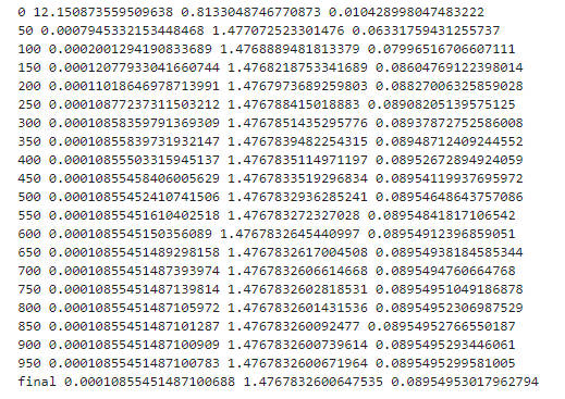
根据输出可以看到最终的 w 和 b 已经无限逼近采样数据模型。
前向传播算法实战
本章节的目标是利用 TensorFlow 的基础数据结构实现解析 MNIST 手写数字数据集问题,与神经网络的计算步骤一致,实现思路如下所示:
1 | # 采用的数据集是 MNIST 手写图片集,输入点数为 784,第一层的输入节点为256,第二层的输入节点为128,第三层的输入节点为10,即样本的属于10类别的概率。 |
AUTO-MPG 汽车油耗
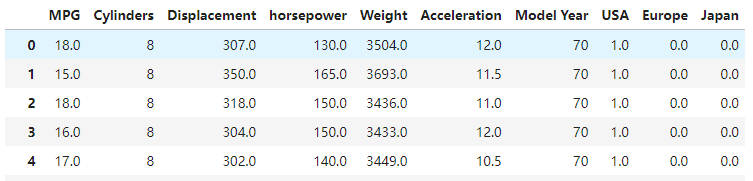
本节将利用全连接网络来训练模型完成预测汽车的效能指标 MPG(Mile Per Gallon,每加仑燃油英里数)。
引入依赖
1 | from tensorflow import keras |
加载数据
1 | # 1. 读取数据 http://archive.ics.uci.edu/ml/machine-learning-databases/auto-mpg/auto-mpg.data |
数据预处理
1 | # 2. 删除空白数据 |
处理模型数据
1 | # 4. 切分训练集和测试集 |
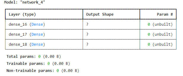
网络模型
1 | # 7. 创建网络 |
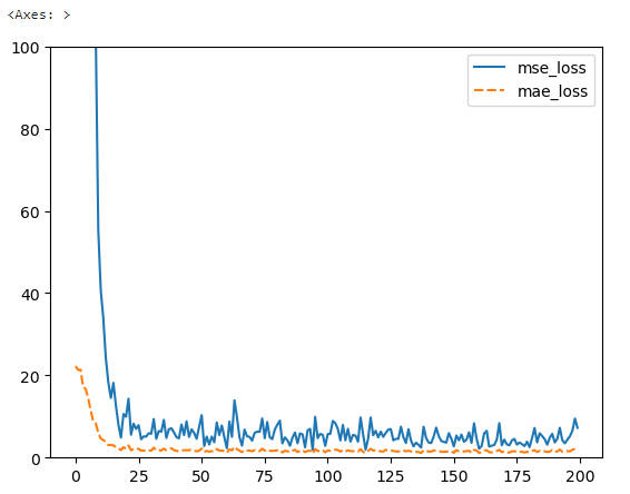
性能指标
1 | # 10. 展示 loss 训练的结果 |
反向传播算法实战
误差反向传播算法(Backpropagation, BP)是神经网络中的核心算法之一。
利用多层全连接网络的梯度推导结果,直接利用循环计算每一层的梯度,并按照梯度下降算法手动更新。
本次推导使用的梯度传播公式是基于多层全连接网络,只有 Sigmoid 一种激活函数,并且损失函数为均方误差函数的网络类型。
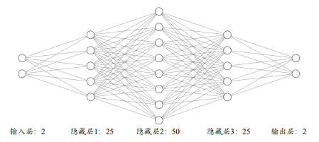
本次将实现一个四层的全连接层网络来完成二分类任务。网络输入节点数为 2,隐藏层的节点数设计为 25, 50, 25,输出层两个节点,分别表示属于类别 1 的概率和类别 2 的概率。
引入依赖
1 | import tensorflow as tf |
数据集
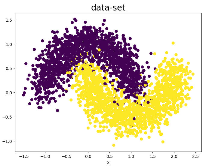
此处使用 sklearn 库提供的工具生成 2000 个线性不可分的二分类数据集,数据的特征长度为 2,采样数据分布如下所示。
1 | N_SAMPLES = 3000 # 采样点数 |
网络层
1 | # 网络层 |
网络模型
1 | # 网络模型 |
网络训练
1 | # 模型训练 |
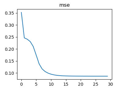
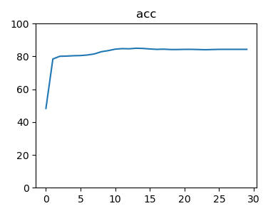
网络性能
1 | # mse 数据图标展示 |
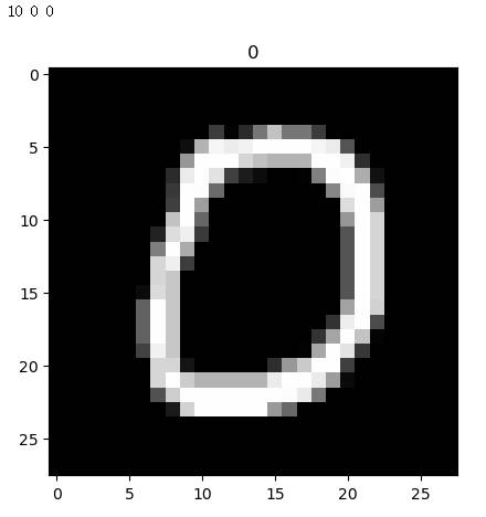
MNIST 数据集
经典机器学习入门实践。
引入依赖
1 | import tensorflow as tf |
加载数据
1 | (x, y), (x_test, y_test) = datasets.mnist.load_data() # x: [60k, 28, 28], [10, 28, 28], y: [60k], [10k] |
处理数据
1 | train_db = tf.data.Dataset.from_tensor_slices((x,y)).batch(128) |
搭建模型逻辑
1 | # [b, 784] => [b, 256] => [b, 128] => [b, 10] |
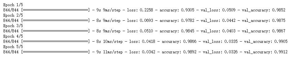
训练模型
1 | for epoch in range(100): # iterate db for 10 |

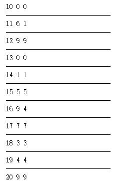
模型验证
1 | # 验证测试集 |
在上述的实例中出现很多第一次出现的内容,这些内容都是卷积神经网络 CNN 中的网络层,不过不用担心,后续会出一篇新的文章去讲卷积神经网络,敬请期待!
总结
俗话说:“实践是检验真理的唯一标准”,而对于机器学习则更加要多多实践!
引用
个人备注
此博客内容均为作者学习《TensorFlow深度学习》所做笔记,侵删!
若转作其他用途,请注明来源!